
Drones are getting faster, and the missions are getting tighter: 15-minute mapping windows, high-speed inspection runs, aggressive turns between waypoints, and gimbals or antenna mounts that swing through large angles while the airframe is still moving. Marketing shorthand reduces all of that to one number — top speed — but GNSS performance in high-dynamics flight is not one number. It is at least two different problems, measured in two different ways.
This article pulls apart three pieces of public evidence that are often quoted together as if they described the same thing: a Septentrio drone mapping case, a peer-reviewed vehicle velocity-estimation study, and an ISRO study of antenna behaviour at high rotation rates. Each is useful. None of them is a product speed rating, and combining their numbers into one claim would be dishonest. What follows is what each source can support, where the boundary sits, and a test protocol you can actually run on your own airframe.
Two Problems Hiding Behind “High-Speed Operation”
Linear dynamics covers speed, acceleration and jerk — how fast the Doppler shift seen by the receiver is changing. It stresses the tracking loops and the navigation filter: can the loop keep lock while the range rate swings, and can the filter stay converged when the platform changes state quickly? You evaluate it with velocity and position error, solution status, and availability over the manoeuvre.
Angular motion covers turns, airframe rotation and the resulting change in antenna orientation. It does not stress the estimation algorithm first — it changes which satellites the antenna can hear at all. You evaluate it with antenna gain patterns, the azimuth/elevation distribution of visible satellites, and whether the receiver can hold continuous tracking long enough to decode orbit data and produce a fix.
Mix the two and you get the classic error: reading a rotation-rate result as if it were a translation speed, or reading a post-processed mapping accuracy as if it were real-time positioning. The table below is the discipline we apply to every source in this article.
| Source | What it actually provides | What it cannot support |
|---|---|---|
| Septentrio UAV mapping case | 7.5 ha / 15 min / 143 photos; offline RTK photo positions; 20 checkpoints better than 3.5 cm in 3D | Not a high-speed test; 3.5 cm is a post-processed photogrammetric result, not real-time flight positioning accuracy |
| Vehicle velocity-estimation paper (2022) | 10 Hz dynamic vehicle test; four velocity algorithms compared across GPS, BDS and GPS+BDS | Not a Septentrio receiver test; velocity error is not position error |
| ISRO high rotation-rate study (2022) | Solution availability versus body rotation rate; antenna pattern versus satellite visibility | Spaceborne/orbital platform study; rotation rate cannot be converted into UAV translation speed |
| Septentrio receiver reference guide | Motion-type and dynamic-level settings, and the response-versus-noise trade-off | Settings and results must be confirmed against the exact model and firmware you deploy |
Evidence 1 — A Septentrio UAV Mapping Case: Efficiency, Not a Speed Benchmark
The case is titled “Look, no Ground Control Points!” and it describes a quarry survey: the site had been closed by a landslide, and the job was to cover roughly 7.5 hectares spread across difficult terrain in a single afternoon. The payload was a high-resolution camera plus a Septentrio AsteRx-m UAS receiver, flown on a pre-planned mission by the autopilot.
| Item | What the case records | How to read it |
|---|---|---|
| Coverage | 7.5 ha (18.53 acres) in a 15-minute flight | That is the mission duration, not a receiver speed or dynamics rating |
| Imagery | 143 photographs | Exposure times time-tagged by camera shutter pulse |
| Onboard logging | Dual-frequency GNSS observations plus shutter events | Provides the observation data and the exposure-time correspondence for post-processing |
| Initial tags | Photos first tagged with single-point positions, typically 1–4 m | Not the final survey product |
| Post-processing | Rover observations combined with base-station files; RTK photo positions computed offline and written back to EXIF | No live base-station datalink has to be maintained during flight |
| Verification | 20 checkpoints; Pix4D and PhotoScan results both better than 3.5 cm in 3D | Checkpoint comparison against the photogrammetric product, not real-time accuracy |
Read as a workflow, the value is a closed loop: plan the mission, capture imagery while logging dual-frequency observations and shutter pulses, align exposures to GNSS epochs, solve RTK offline against the base station, then verify with independent checkpoints instead of trusting the software’s own report. Dropping ground control points is what made a landslide-closed site workable in one afternoon.
For a UAV operator the takeaway is efficiency and data hygiene, not speed. If you quote this case on a product page, quote it as a mission-workflow result with its preconditions — dual-frequency observations, shutter synchronisation, base-station data, offline RTK — and never as airborne real-time accuracy.
Evidence 2 — 10 Hz Vehicle Velocity Estimation: What Four Algorithms Deliver
The second source is a peer-reviewed study: Li Ji, Rui Sun, Qi Cheng and Junhui Wang, “Evaluation of the performance of GNSS-based velocity estimation algorithms”, Satellite Navigation 3, 18 (2022), open access under CC BY 4.0. It asks a narrow, useful question: across static, dynamic, open-sky and urban environments, how do different observation types and processing strategies compare for velocity estimation? Note two boundaries before any number is reused: the dynamic test used a 10 Hz multi-frequency receiver that is not a Septentrio product, and the reported quantities are velocity component errors in m/s.
| Element | As described in the paper |
|---|---|
| Receiver / rate | 10 Hz multi-frequency GNSS receiver (not a Septentrio product) |
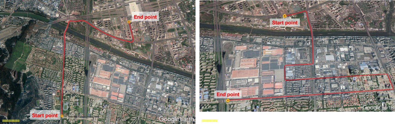
| Test 1 route | Wide arterial roads in Nanjing, lightly urbanised environment |
| Test 2 route | Moderate urban canyon, taller buildings, heavier masking and reflection |
| Reference velocity | Post-processed tightly coupled high-grade IMU + RTK GNSS system |
| Methods compared | Raw Doppler (RD), time-differenced pseudorange (TDPR), time-differenced carrier phase (TDCP), double-differenced carrier phase (DDCP) |
| Constellations | GPS, BDS, and GPS+BDS |
| Method | Information used | Behaviour reported |
|---|---|---|
| RD — raw Doppler | Current-epoch Doppler and pseudorange rate | Responds directly to rapid state changes; described as performing well under high dynamics |
| TDPR — time-differenced pseudorange | Pseudorange change between adjacent epochs | Simple, but urban multipath amplifies the error; the weakest of the four in the dynamic tests |
| TDCP — time-differenced carrier phase | Carrier-phase change between adjacent epochs | High precision; continuity suffers when signals are interrupted or lost |
| DDCP — double-differenced carrier phase | Carrier phase differenced across satellites and epochs | High precision but needs enough satellites and continuous observations; masking reduces availability |
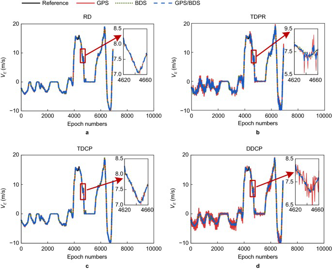
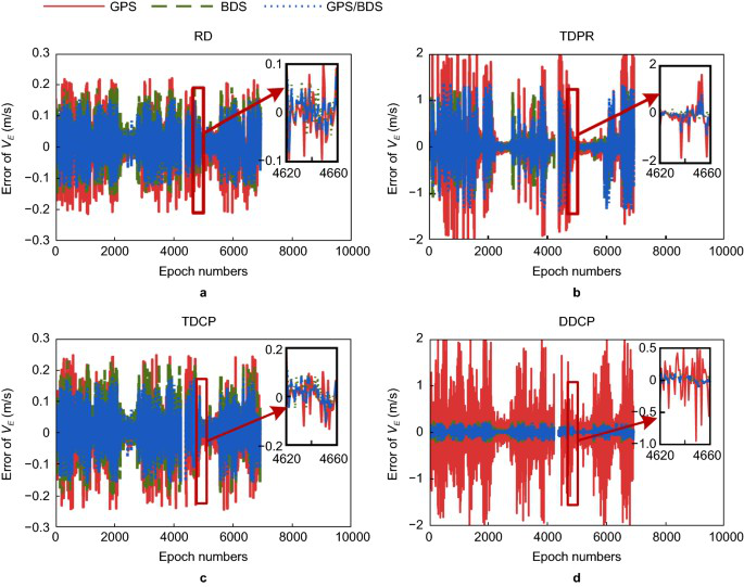
Test 1 results (open arterial roads). The velocity traces show a distinct deceleration-then-acceleration segment, which the authors enlarge around epochs 4620–4660. RD tracks the reference most closely; the other methods drift and ripple around it.
| Metric | Reported value | Reading |
|---|---|---|
| Rate / reference | 10 Hz; IMU + RTK reference, post-processed | Dynamic vehicle test, not a static bench |
| BDS + RD RMSE | East 0.051 m/s; North 0.077 m/s; Up 0.147 m/s | Velocity error; the vertical component is the largest |
| BDS + TDCP / DDCP RMSE | East and North below 0.1 m/s; Up below 0.2 m/s | Range figures given in the paper text |
| BDS + TDPR RMSE | East 0.173 m/s; North 0.341 m/s; Up 0.857 m/s | Clearly worse than RD, TDCP and DDCP in this test |
| TDPR maximum error | BDS: East 1.280 m/s, North 2.789 m/s, Up 7.125 m/s | Large outliers remain; the authors link them to pseudorange error and multipath |
| Maximum error, other three | RD, TDCP and DDCP all within 1 m/s | As described for this dynamic test |
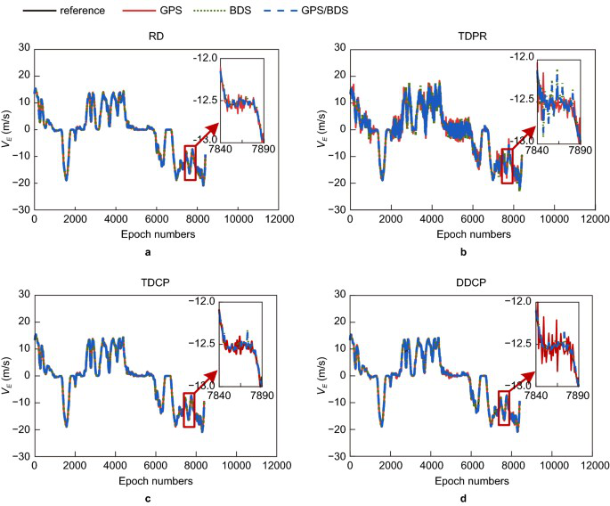
Test 2 results (urban canyon). With taller buildings, masking and reflection dominate. RD, TDCP and DDCP land roughly in the 0.1–0.2 m/s band; TDPR spreads from decimetres to metres per second. GPS+BDS tracks the reference better overall and suppresses the spikes — but availability, not just accuracy, separates the constellations.
| Metric | GPS | BDS | Reading |
|---|---|---|---|
| RD horizontal RMSE, East | 0.104 m/s | 0.081 m/s | Lower for BDS in this test |
| RD horizontal RMSE, North | 0.142 m/s | 0.085 m/s | Lower for BDS in this test |
| RD maximum horizontal error, East | 0.462 m/s | 0.442 m/s | Lower for BDS |
| RD maximum horizontal error, North | 0.728 m/s | 0.476 m/s | Lower for BDS |
| DDCP continuous availability | 77.14% | 96.60% | More BDS satellites meant more epochs satisfied DDCP’s satellite requirement; GPS+BDS improved availability further, though the paper does not quote the combined percentage here |
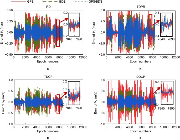
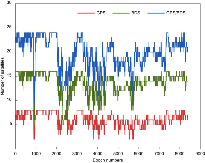
The transferable idea is the test design, not any single figure: state the update rate, the reference system, the route environment, the motion profile, the error statistic and the availability, and report horizontal and vertical components separately. That is exactly the discipline a drone GNSS evaluation needs.
Evidence 3 — ISRO’s Rotation-Rate Study: Angular Motion Is a Separate Failure Mode
The third source comes from the ISRO Inertial Systems Unit: “Impact of Radiation Pattern of GNSS Receiver Patch Antenna in positioning during high rotation rate & Mitigation Techniques”, URSI-RCRS 2022. It concerns launch-vehicle and orbital platforms, not multirotors, and its central finding is precisely the distinction this article is built on: a receiver’s linear-dynamics capability and its ability to hold satellites while the platform rotates are two different things.
| Item | As reported |
|---|---|
| Antenna arrangement | Two antennas 180° apart on the body, each with its own LNA, combined by a power combiner into a single receiver front end |
| Frequencies | GPS L1 1575.42 MHz; NavIC L5 1176.45 MHz |
| Antenna type | Stacked circularly polarised microstrip patch, RHCP, 50 Ω |
| Selected specs | Typical gain 3 dBic; bandwidth (RL > 10 dB) about ±5 MHz; return loss ≥ 14 dB; axial ratio ≤ 5 dB |
| Pattern | Peaks near azimuth 0° and 180° at low elevation; satellites need to sit roughly within ±70° azimuth/elevation to be received well |
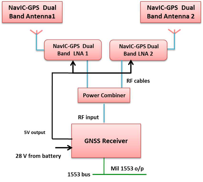
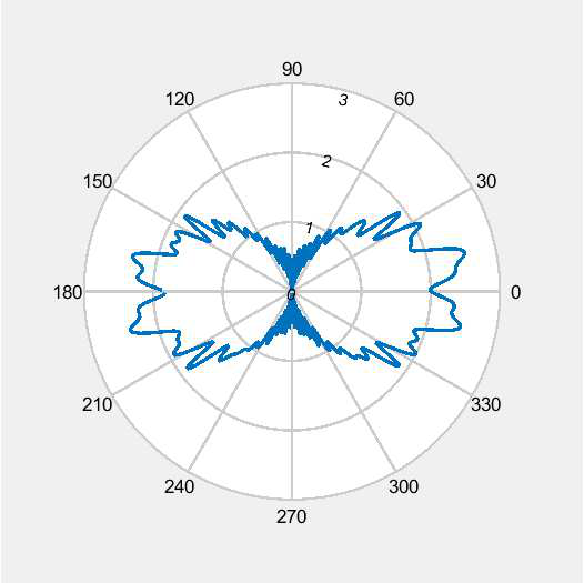
The tracking prerequisites matter more than the pattern for a UAV reader. Before a satellite can contribute to a solution, the receiver must collect its ephemeris and decode satellite time. The report gives GPS ephemeris 18–36 s and NavIC 24–60 s, GPS time-of-week 12–18 s and NavIC 24–36 s, after which at least four such satellites must be tracked continuously for about a second to compute a fix. Any short loss of lock during rotation therefore hits solution continuity directly.
From a 140° continuous-tracking azimuth window and the GPS 12–18 s requirement, the paper derives an upper bound of about 7.78°/s (roughly 7°/s) for single-axis rotation, then tests it with a GNSS RF signal simulator and flight-representative hardware. The measured availability is blunt:
| Test condition (single axis) | Body rate | Solution availability | Note |
|---|---|---|---|
| Roll | 0.5°/s | 97.88% | Essentially usable |
| Roll | 1°/s | 97.21% | Essentially usable |
| Roll | 2°/s | 97.01% | Essentially usable |
| Roll | 5°/s | 69.40% | Positioning clearly degraded |
| Roll | 7°/s | 59.28% | Positioning clearly degraded |
| Roll | 8°/s | 0% | No solution |
| Roll | 10°/s | 0% | No solution |
| Tri-axis orbital condition | Solution availability | Note |
|---|---|---|
| 2°/s | 96.38% | High availability |
| 5°/s | 74.62% | Availability drops |
| 6°/s | 6.78% | Severely affected |
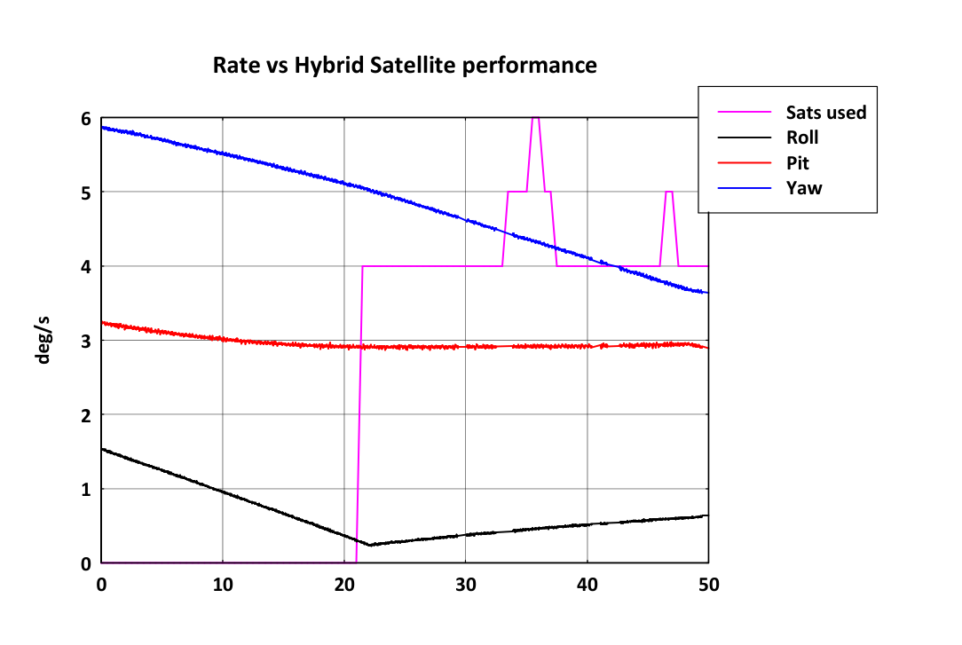
In the orbital test the initial rates were about 6°/s yaw, 3°/s pitch and 1°/s roll; there was no usable solution at the high-rate stage, and the solution recovered roughly 20 seconds later once yaw fell below 5°/s. The paper also evaluates antenna mitigation: three antennas at 120° spacing perform worse because their patterns interfere, while four antennas at 90° split into two groups feeding independent RF front ends is proposed as a potential fix — explicitly still under verification, not a settled product conclusion.
For drone work, quote it the way it is written: airframe rotation and antenna pattern affect whether satellites stay continuously visible. Do not turn 7°/s into a flyable speed. It is a rotation rate measured on an orbital platform with a specific antenna configuration.
What Septentrio’s Motion and Dynamic Level Settings Really Trade Off
Septentrio’s AsteRx SB3 Pro+ reference guide (firmware v4.10.1) exposes the practical lever for dynamic platforms. Motion tells the receiver what kind of motion to expect — UAV, RaceCar, Automotive and similar profiles — so the navigation filter matches the platform. Level balances response against noise: the guide recommends keeping the adaptive Moderate setting in normal use, and raising the level when you need shock, vibration or fast displacement to show up in the output, accepting more noise. Max disables the navigation filter and computes each epoch independently, which is the most responsive setting but can increase PVT output latency.
| Setting | Options | Behaviour and cost |
|---|---|---|
| Motion | UAV / RaceCar / Automotive, etc. | Matches the filter’s dynamic model to the platform’s expected motion |
| Level | Moderate (recommended default), higher levels, Max | Higher levels expose high-frequency dynamics but raise position noise |
| Level = Max | Navigation filter disabled, per-epoch solution | Fastest response, noisier output, possible increase in PVT latency |
So “crank up the dynamics” is not a strategy. The setting has to match the airframe, the vibration environment, the required output rate and the latency the flight controller can tolerate — and it has to be confirmed against the exact Septentrio model and firmware you are deploying, not a guide written for a different product.
A Test Protocol You Can Run on Your Own Airframe
- Record the configuration first: receiver model and firmware, antenna model and mounting position, update and output rates, and every Motion/Level setting you changed.
- Fly the manoeuvre, not a hover: capture the acceleration, deceleration, turn and vibration profile you actually care about, with timestamps.
- Log solution status continuously: fix type, number of satellites, solution availability percentage, and the exact times of any loss of lock and recovery.
- Measure latency: PVT output delay and jitter at your configured rate, since a fast solution that arrives late is not usable for control.
- Use an independent reference: a separate IMU/RTK truth system, and report horizontal and vertical error separately as RMSE and maximum error, with sample counts and the time window.
- Separate the two dynamics: report linear speed/acceleration results apart from body rotation rates and antenna orientation, and never convert one into the other.
Hardware for High-Dynamics UAV Work: HB56 and HB56H
If the mission profile is demanding, the receiver has to be chosen for it rather than tuned into it. Two UAV GNSS receivers cover the two halves of the problem above:
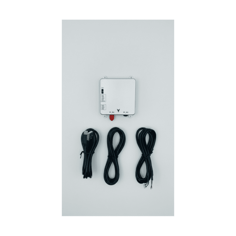
- HB56 multi-frequency GNSS receiver — built on the Septentrio mosaic-X5 module. This is the workhorse for high-rate position and velocity on a moving platform: multi-frequency, multi-constellation tracking, with the module’s onboard anti-jamming and interference mitigation. Choose it when the mission needs a compact receiver that can log observations at high output rates for PPK or RTK workflows.
- HB56H dual-antenna GNSS heading receiver — built on the Septentrio mosaic-H module, using two antennas to give true heading as well as position. Choose it when rotation is part of the mission — gimbal sweep, tight turns, antenna orientation changes — because heading from two widely separated antennas is far more stable than a course-over-ground value derived from consecutive positions.
The pairing is deliberate: HB56 answers the linear-dynamics question with a mosaic-X5 core, and HB56H answers the orientation question with mosaic-H and its dual-antenna baseline. For a test campaign, run the same route and the same Motion/Level configuration on each, then compare availability, latency and horizontal/vertical error against your reference — that is the data a selection decision should rest on.
FAQ
Does a receiver’s maximum velocity spec prove it works at high speed?
No. A velocity limit describes one part of linear-dynamics capability — that the tracking loop can follow the Doppler rate in that range. It says nothing about turns, vibration, masking, urban multipath, output latency or solution availability, and a UAV evaluation has to cover all of those on the real airframe.
Can 7.5 hectares in 15 minutes be converted into a drone speed or an accuracy figure?
No. Area covered and flight time come from mission planning, image overlap, battery endurance and airspace constraints, not from the receiver. And the better-than-3.5 cm figure in that case comes from post-processed photogrammetry checked against 20 ground points, not from real-time positioning during the flight.
The velocity paper reports 0.051 m/s — is that a centimetre-level positioning accuracy?
No. That number is a velocity component error, east component, for one algorithm and one constellation in one test. Position accuracy needs a position reference and position error statistics. Converting m/s errors into centimetres of position accuracy is a category error.
Does the ISRO rotation study mean a drone cannot fly at 7°/s?
No. That number is an angular rate derived from a specific antenna configuration and tracking-window analysis on orbital hardware. It tells you that rotation rate and satellite visibility are coupled, and that availability collapses quickly past a threshold. It is not a translation speed and not a drone flight limit.
Should I just set the dynamic level to Max for aggressive flight?
Usually not as a default. Max disables the navigation filter and outputs an independent solution each epoch: very responsive, but noisier and potentially higher latency. Higher levels are a trade, not a free upgrade. Raise the level only when your logged data shows the platform’s dynamics are being smoothed away, and check the result against a reference.
What should I log to prove GNSS performance in high-dynamics flight?
Model and firmware, antenna and mounting, update and output rates, the Motion/Level settings, the speed and body-rate profile, solution status and availability with loss-of-lock and recovery times, PVT latency, and horizontal/vertical error against an independent reference — as RMSE and maximum error, with sample counts and the time window.
Sources and Figure Credits
Septentrio mapping case: “Look, no Ground Control Points!”, AsteRx-m UAS case page, Septentrio — septentrio.com.
Velocity estimation paper: Ji, L., Sun, R., Cheng, Q., & Wang, J. (2022). Evaluation of the performance of GNSS-based velocity estimation algorithms. Satellite Navigation, 3, 18. Open access, CC BY 4.0 — doi.org/10.1186/s43020-022-00080-4.
Rotation-rate study: Mohammed Basim A. et al. (2022). Impact of Radiation Pattern of GNSS Receiver Patch Antenna in positioning during high rotation rate & Mitigation Techniques. URSI-RCRS 2022 — ursi.org proceedings.
Receiver settings: Septentrio, AsteRx SB3 Pro+ Reference Guide, firmware v4.10.1 — reference guide (PDF).
Figure credits: figures 1–6 are reproduced from the open-access Satellite Navigation paper under CC BY 4.0 with attribution; figures 7–9 are selected figures from the URSI-RCRS 2022 paper. Confirm licensing with the original publishers before any commercial reuse.
Related Reading
- GNSS attitude from a moving base: dual-antenna RTK for UAVs — how two antennas produce heading while the platform moves.
- Multipath, jamming and 100 Hz: GNSS in motion — what high-rate output looks like under real interference.